| Midway Physics Day Ride Analyses |
| Drop of Fear |
| Himalaya |
| Enterprise |
| Ferris Wheel |
| Rainbow |
| Starship 2000 |
| Swing Chairs |
| Wild Cat Roller Coaster |
| Home |
Drop of Fear
G. Robertson, D. Tedeschi
University of South Carolina

| Midway Physics Day Ride Analyses |
| Drop of Fear |
| Himalaya |
| Enterprise |
| Ferris Wheel |
| Rainbow |
| Starship 2000 |
| Swing Chairs |
| Wild Cat Roller Coaster |
| Home |
Drop of Fear
G. Robertson, D. Tedeschi
University of South Carolina
Introduction:
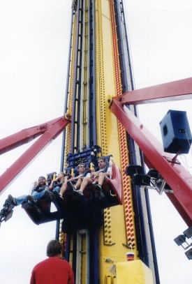
The “Drop of Fear” is a ride at Midway physics day in which a person rides a platform which lifts them to a certain height (around 55 meters) and then drops the platform so that the rider is in free-fall for about 2 seconds. The ride then brakes and comes to a stop. The data taken from this ride was gathered with the help of a single axis, accelerometer, a barometer and a CBL. The accelerometer has an axis that when pointed upwards (under normal circumstances) will give a reading of –9.81 m/s2; when the axis is pointed downward, like in this data, the reading is a positive 9.81 m/s2. The barometer was used to measure the air pressure at points along the ride. By taking a reference pressure (around 1029 mm-Hg), subtracting it by the pressure measured, and then dividing that by the conversion of 0.0864 mm-Hg/m, the height of the rider could be found easily.
Weight, commonly measured in Newtons, is usually considered as W= mg , but for the Drop of Fear, the system is accelerating, and weight must be considered as the reading given by an accelerometer in the accelerating system. The following free-body diagram illustrates this idea. The reading on the accelerometer is the Normal Force, N.

![]()

Ride Data:
In the graph above, the data for the ride, “The Drop of Fear,” is shown plotted as acceleration and height against time. At 23 seconds, the ride has reached its peak altitude of around 55 meters and the acceleration felt by the rider is at a constant 9.81 m/s2. From a little after 25 seconds to 27.75 seconds, the rider is in free-fall and the height is plummeting towards 0 meters. After 27.75 seconds however, the ride begins braking and the riders feel a maximum acceleration of about 4 g’s! The ride quits braking after 30 seconds and the ride is over.
Velocity:
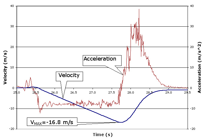
In this graph, the data is plotted as velocity and acceleration over time. The following kinematics equation was used to calculate the velocity on the ride at every point using a Microsoft Excel spreadsheet.
![]()
It is seen in the graph that the velocity peaks to –16.8 meters per second during the time that the riders are in free-fall, this can be compared to the value of 19.62 meters per second given by vf = at, using the average acceleration due to gravity, -9.81m/s^2, over the period of free fall of 2 seconds: (-9.81m/s^2)(2s)= -19.62 m/s.
Position:
While there was already a device used to calculate the height of the rider, the accelerometer can also be used to calculate this height using the previous calculated instantaneous velocities and the following kinematics equation:
![]()
The following graph shows the height calculated using the method mentioned above and compares it to the height as calculated by the barometer reading.
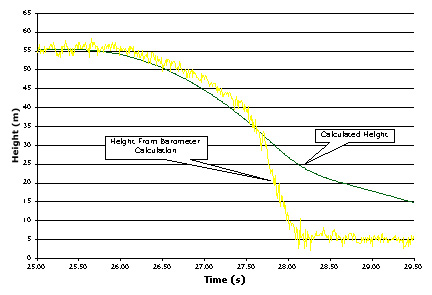
The difference in the two graphs is due mostly to the axis in the accelerometer not being pointed straight down. If the axis was tilted slightly, or moved during the ride (which is what seems to have happened), then the graph would deviate from the height calculated from the barometer measurements. Also, the calculation of this height is only valid when the acceleration is constant, as shown previously, there is a very large change in acceleration and that provides a reason for the large deviation after 27.5 seconds. However, during the time of free-fall (about 25.5 seconds to around 27.5 seconds) the calculated height predicts the barometric height well.
Advanced Analysis:
The impulse-linear momentum theorem states that pf - pi =Dp= J= FDt. We can test this theorem on the Drop of Fear data.
Because the initial and final velocities are both zero, the change in momentum must also be zero.
![]()

Using this information, it should be clear that the sums of the two shaded regions on the graph below should equal zero.
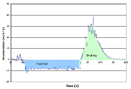
To calculate the area within the shaded regions of the graph, the following methods were used to numerically integrate the regions in Microsoft Excel:
|
Method
|
Equation
|
Area 1
|
Area 2
|
|
2-Point Equation
|
|
-16.7
|
16.2
|
|
Simpson's Rule
|
|
-16.6
|
16.1
|
|
Trapezoidal Rule
|
|
-16.6
|
16.1
|
All of the acceleration data points were subtracted by 8m/s2 (gravity, as measured by the accelerometer) in order to achieve the most precise results.